
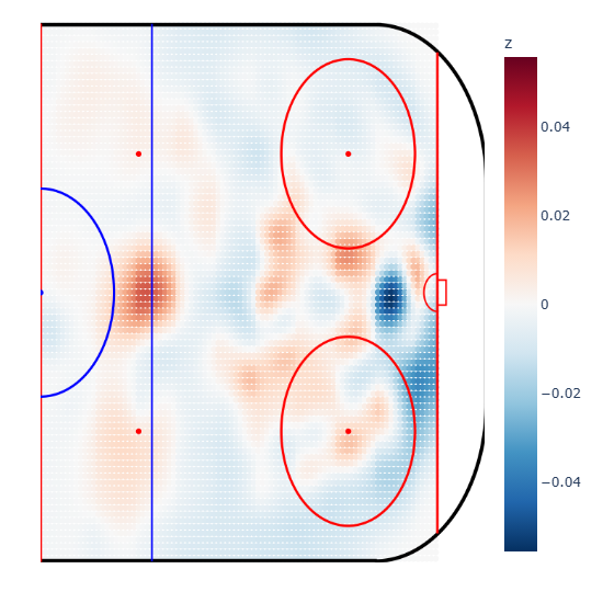
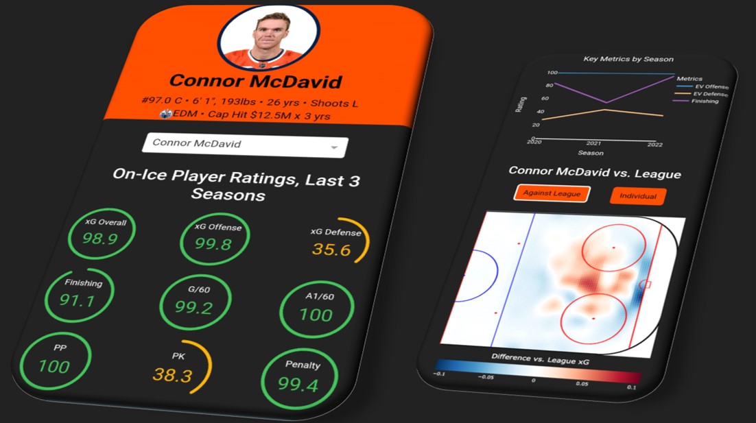
A per-player even-strength xG heatmap (Connor McDavid vs. league) - the kind of output the model produces, rendered in the datarena app.
Machine Learning
Building a calibrated NHL xG model
A deep-dive on the expected-goals model behind datarena - calibration, temporal validation, and walk-forward scoring.
This is the technical companion to datarena. If the main write-up is the what, this is the how - the expected-goals model that everything else in the platform exists to serve.
I built this the way I’d build a model at work: temporal validation, calibration as a first-class concern, an A/B to justify the architecture, and full experiment tracking. It’s a hobby project on public data, but I wanted to hold it to the same standard.
Expected Goals (xG) estimates the probability that a given shot becomes a goal. Sum it up, and you can measure how many goals a player or team should have scored or allowed - a far more stable signal than goals alone.
Table of Contents
- Problem framing
- Data & temporal split
- Features
- Model & calibration
- One model, not three
- Walk-forward scoring
- Results & honesty
Problem framing
| xG is **P(goal | unblocked shot)** - a binary classification on a shot-level table, where the positive class (goals) is only ~7.2% of shots. The scope is Fenwick shots (goals, shots on goal, and missed shots); blocked shots and shootouts are excluded upstream. |
The critical constraint: the output has to be a calibrated probability, not just a good ranking. xG gets summed across players, games, and seasons, so an xG of 0.2 must genuinely correspond to a ~20% goal rate. A model that ranks shots perfectly but is miscalibrated is useless here. That reframes the whole problem around proper scoring and calibration rather than accuracy or AUC.
Data & temporal split
Features come from a dbt-owned shot table (fct_shot) - the ML repo deliberately does no feature engineering, so there’s one source of truth for what each feature means. The split is strictly temporal:
| Split | Seasons | Role |
|---|---|---|
| Train | 2020-21 → 2023-24 | Fit the booster |
| Validation | 2024-25 | Early stopping and calibration |
| Test | 2025-26 | Untouched final evaluation |
Why temporal and never random? Shots are time-ordered, and a random split leaks game- and season-level context across train and test, inflating every metric. Training on the past and evaluating on a held-out future season measures honest forecasting skill - which is exactly how the model is used in production.
Features
21 leakage-safe features, all sourced from the warehouse:
| Family | Examples |
|---|---|
| Geometry | shot distance, angle, type, side, off-wing |
| Sequence | is-rebound, is-rush, time since last event/shot, previous event type |
| Game state | score for/against, score differential, strength state, empty net, skater counts |
| Context | shooter handedness, team side, period |
Categoricals are handled natively (XGBoost’s enable_categorical), with training category levels persisted so scoring stays aligned. A couple of deliberate exclusions tell the story of how careful you have to be:
event_typeis excluded - it is the outcome (event_type = 'goal'⟺ the label). Including it is textbook leakage.- The pre-shot score features were briefly pulled when an upstream bug left them NULL on every non-goal - the nullness itself leaked the label and sent ROC-AUC to a suspicious 1.0. Once fixed, they came back. (That moment - “why is my AUC perfect?” - is a good reminder that leakage usually looks like great results.)
Model & calibration
Gradient-boosted trees (XGBoost). Tabular, heterogeneous features with non-linear interactions and a noisy target - GBDTs are the right default, and they beat linear and naive-distance baselines.
The hyperparameters are unremarkable on purpose (max_depth=6, learning_rate=0.03, up to 2000 trees with early stopping on the validation season landing around 400). The interesting choices are about probabilities:
- No
scale_pos_weight. Reweighting the 7% positive class is the usual reflex for imbalance, but it distorts the output probabilities. I keep the true priors and fix the rate with calibration instead - a deliberate calibration-first decision. - Isotonic calibration, fit on the validation season (out-of-training, so the calibrated probabilities aren’t optimistic). Raw boosted scores rank well but aren’t a true rate; isotonic maps them onto observed goal rates.
One model, not three
The legacy approach trained three models split by strength state (even-strength / powerplay / penalty-kill), and in isolation each looked strong. I A/B’d that against a single unified model with strength state as a feature - same features, same temporal holdout:
| Model | ROC-AUC | log-loss | Brier | ECE |
|---|---|---|---|---|
| Unified | 0.7663 | 0.2238 | 0.0607 | 0.0046 |
| 3-split | 0.7645 | 0.2258 | 0.0609 | 0.0049 |
The unified model won overall and within every strength state. Why: gradient boosting learns goal geometry that’s mostly shared across strengths, so one model trains on all ~445k shots while the split starves the powerplay (~20k) and penalty-kill (~3.7k) sub-models of data. With strength as a feature, the unified model still specializes where it helps - and there’s one artifact to calibrate, version, and serve instead of three.
The lesson I took from this: the legacy split looked better partly because it was reporting per-stratum metrics on low-base-rate subsets (an EV-only log-loss is naturally lower than an all-shots number) and using an optimistic random split. On an apples-to-apples comparison, it didn’t win. Always compare on the same held-out shots.
Walk-forward scoring
A single train/test split is how you develop and pick a recipe. But the app needs an xG on every shot across 13 seasons, and goal-scoring is non-stationary - equipment, rules, and scoring trends drift. Scoring a 2014 shot with a model trained on 2024 data injects future information into the past.
So production scoring uses walk-forward (rolling-origin): for each target season, train on a window of seasons strictly before it, calibrate on the most-recent prior season, then score it. Every season is out-of-sample for its own model - leakage-free, and the recipe respects drift.
I didn’t guess the window length, I measured it:
| Target season | Expanding (all prior) | Trailing-3 |
|---|---|---|
| 2025-26 | 0.766 | 0.776 |
Dropping the oldest seasons helped - recency matters, and the anomalous COVID/bubble 2020-21 season actively hurt. So the default is a trailing ~3-season window, configurable and re-measured as the data deepens. The backfill currently produces xG for 2013-14 → 2025-26, each season scored by its own vintage with full provenance (model version, training window, scored-at).
Everything runs through MLflow - every run logs params, metrics, a reliability plot, and feature importances, and serving is pinned to a model alias so a retrain never silently changes the xG that’s already published.
Results & honesty
On the held-out 2025-26 test season (calibrated): ROC-AUC 0.766, log-loss 0.224, Brier 0.061, ECE 0.005.
I want to be straight about what that means. A ROC-AUC around 0.77 is in line with public xG models - hockey is high-variance and a shot’s outcome is genuinely close to a coin-weighted-by-geometry, so there’s a real ceiling here. The number I actually care about is the ECE of ~0.005: the probabilities are trustworthy, which is the entire point of an xG model. Chasing a higher AUC by adding leaky features would make the model look better and be worse.
There’s plenty left to build - on-ice/WOWY features, a hyperparameter sweep, SHAP artifacts per run, monotonic constraints on distance - and it’s all tracked openly. But the foundation is the part I’m happy with: it’s calibrated, it’s leakage-safe, it’s reproducible, and every architectural choice was made on evidence rather than vibes.
If you build probability models for a living and want to talk shop, reach out - this is my favorite kind of conversation. Back to the datarena overview.
Next
Data Science & Machine Learning
datarena.app
An end-to-end NHL analytics platform - from raw API to a calibrated xG model and a live app.